Fundamentals | 18 min read | Intermediate
Simon's Two-Stage Design: A Worked Example for a Phase II Clinical Trial
Follow a worked Simon's two-stage design example with p₀ = 0.10 and p₁ = 0.30: translate clinical assumptions into a decision rule, compare Optimal, Minimax and Admissible designs, and calculate PET, expected sample size, Type I error and power.
Define the Clinical Scenario
Imagine you are planning a single-arm Phase II clinical trial to evaluate a new treatment for patients with advanced cancer. The treatment is promising, but you do not yet know whether its response rate is high enough to justify further development.
Your clinical team considers a response rate of 10% or less unacceptable. A response rate of 30% or higher would be sufficiently promising to warrant further investigation.
You need to decide how many patients to enroll before the first assessment, how many responses are needed to continue, how many additional patients to enroll, the maximum number of patients required, how likely the trial is to stop early if the treatment is ineffective, and which design offers the best balance between patient exposure and recruitment requirements.
A Simon's two-stage design addresses these questions by allowing a trial to stop early for futility. In this worked example we translate clinical assumptions into statistical parameters, generate candidate designs, compare their operating characteristics, and select a design based on practical trial requirements. If you want the methodology first, start with Simon's two-stage design explained.
The primary endpoint is objective response rate (ORR), defined as the proportion of patients achieving a complete or partial response according to the trial’s prespecified response criteria.
The objective is to test whether the treatment has sufficient activity to justify further development. This is a screening decision, not a definitive demonstration of clinical benefit. A Simon's two-stage design suits this setting because it provides an opportunity to stop the trial early when the observed response rate is insufficiently promising.
The clinical team agrees on two response-rate thresholds:
| Parameter | Value | Clinical interpretation |
|---|---|---|
| Unacceptable response rate | 10% | The treatment is not sufficiently active |
| Promising response rate | 30% | The treatment has sufficient activity to warrant further investigation |
Specify the Statistical Parameters
The classical Simon's two-stage design tests H₀: p ≤ p₀ against H₁: p ≥ p₁, where p₀ is the unacceptable response rate and p₁ is the promising response rate. For this example, p₀ = 0.10 and p₁ = 0.30.
You must also specify the acceptable Type I error and the desired power. We will use:
| Design parameter | Value | Meaning |
|---|---|---|
| p₀ | 0.10 | Unacceptable response rate |
| p₁ | 0.30 | Promising response rate |
| Type I error (α) | 0.05 | Maximum probability of incorrectly declaring the treatment promising under the null hypothesis |
| Power (1 − β) | 0.80 | Desired probability of declaring the treatment promising when the true response rate is 30% |
Understand the Two-Stage Decision Rule
A Simon's two-stage design is commonly represented by five numbers: n₁, the number of patients enrolled in Stage 1; r₁, the maximum number of Stage 1 responses that leads to stopping for futility; n₂, the number of additional patients enrolled in Stage 2; N, the maximum total sample size; and r, the maximum total number of responses for which the treatment is not declared promising.
Since N = n₁ + n₂, only four of these values are independent. Together, they describe the sample sizes and the two decision thresholds that determine whether the trial stops early or continues, and whether the treatment is ultimately declared promising.
After Stage 1, if the number of responses is less than or equal to r₁, stop the trial for futility; if it exceeds r₁, continue to Stage 2. After Stage 2, if the total number of responses is greater than r, declare the treatment promising; otherwise, do not.
For example, a design with n₁ = 10 and r₁ = 1 means that 0 or 1 response among the first 10 patients stops the trial for futility, and 2 or more responses lead to enrolling the additional Stage 2 patients. The final response threshold is a separate part of the decision rule.
Generate Candidate Designs
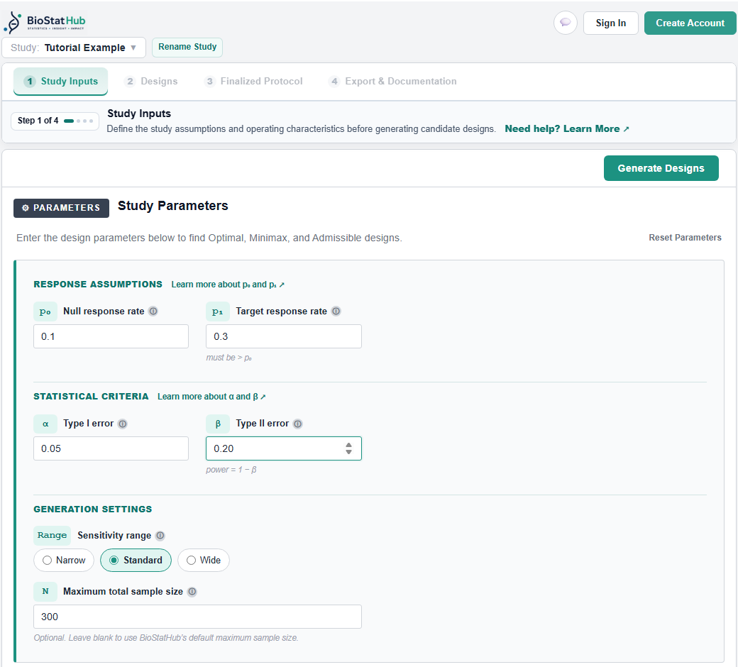
With the clinical and statistical assumptions defined, you can generate candidate designs. Create a study in BioStatHub and enter the four assumptions in the Study Parameters panel. BioStatHub asks for the Type II error β = 0.20 and displays the resulting power, 1 − β = 0.80, beneath the field.
Then select Generate Designs. BioStatHub searches every two-stage decision rule that satisfies the Type I error and power constraints, up to the maximum total sample size, and returns the Optimal and Minimax designs together with the Admissible designs between them.
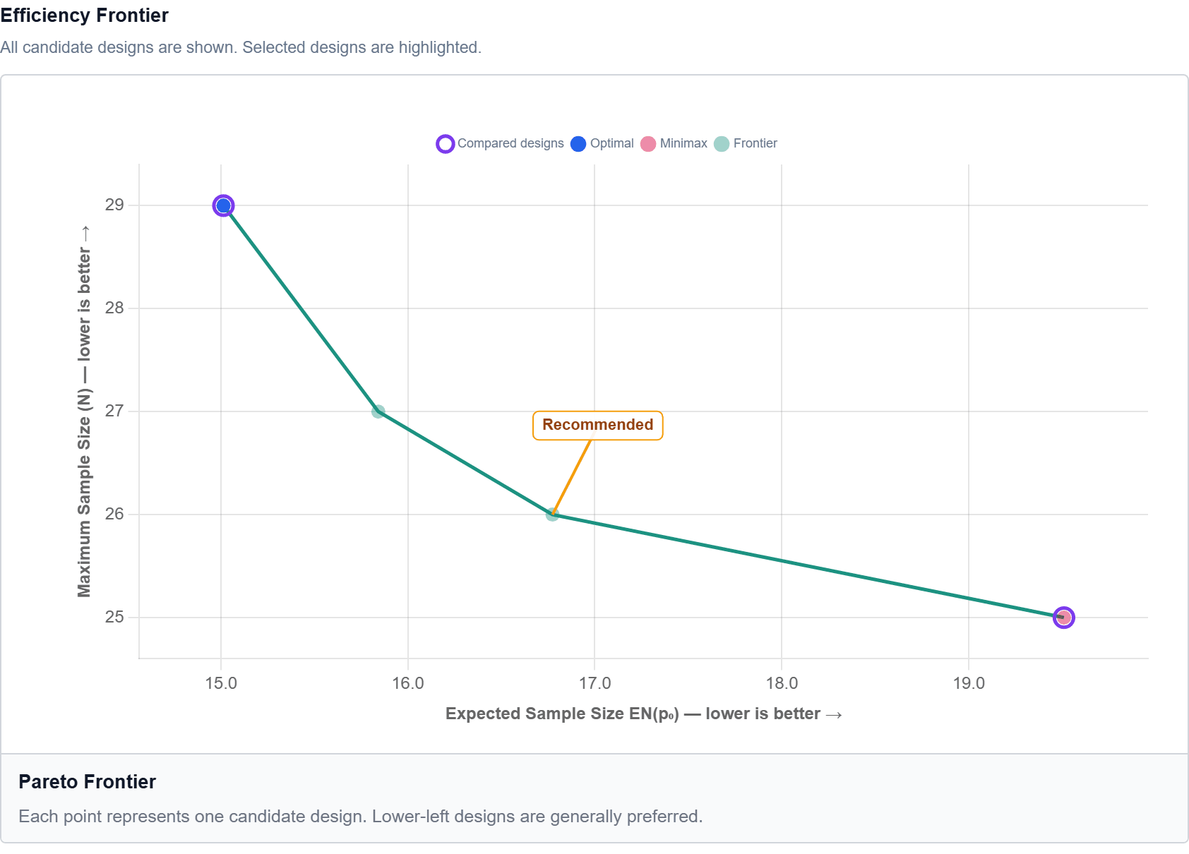
The resulting designs differ in their first-stage sample sizes, maximum sample sizes, expected sample sizes, and probabilities of early termination. There is not necessarily one uniquely best Simon design: different designs can satisfy the same statistical requirements while making different trade-offs.
Compare the Numerical Results and Trade-offs
For the assumptions in this example, BioStatHub returns four candidate designs:
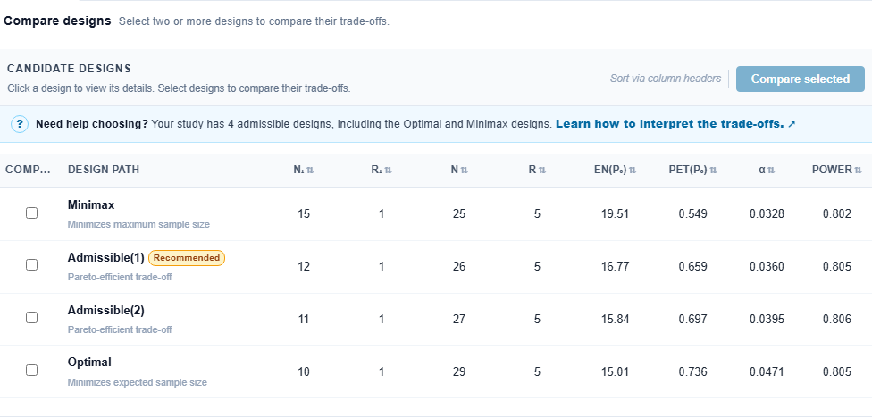
| Design | n₁ / r₁ | N / r | EN(p₀) | PET(p₀) |
|---|---|---|---|---|
| Minimax | 15 / 1 | 25 / 5 | 19.51 | 0.5490 |
| Admissible(1) | 12 / 1 | 26 / 5 | 16.77 | 0.6590 |
| Admissible(2) | 11 / 1 | 27 / 5 | 15.84 | 0.6974 |
| Optimal | 10 / 1 | 29 / 5 | 15.01 | 0.7361 |
Reading the trade-off
Each design is written as n₁ / r₁ for Stage 1 and N / r overall, the notation BioStatHub uses. The Stage 2 sample sizes n₂ = N − n₁ are 10, 14, 16 and 19 patients respectively. Every design has r = 5, so success requires at least 6 responses.
The table illustrates the trade-off between maximum sample size and expected sample size under the null hypothesis. The Minimax design has the smallest maximum sample size, 25 patients. The Optimal design has the smallest expected sample size under the null hypothesis, approximately 15.01 patients. The Admissible designs provide alternatives between these two extremes.
The Optimal design requires a maximum of 29 patients, compared with 25 for the Minimax design, but it has a lower expected sample size when the true response rate is 10%. This is why comparing maximum sample size alone can be misleading.
What does Admissible mean?
Following Jung et al. (2004), a design is admissible if it minimizes a weighted average of the maximum sample size and the expected sample size under p₀, q × N + (1 − q) × EN(p₀), for some weight q between 0 and 1. A weight of q = 1 gives the Minimax design and q = 0 gives the Optimal design. An admissible design is therefore never dominated: no other feasible design is at least as good on both N and EN(p₀) and strictly better on one.
For this example, the two Admissible designs are the complete set BioStatHub returns between the Minimax and Optimal designs. Other software can report a different set if it uses a different search range, tie-breaking rule, or definition of admissibility, so check the convention when comparing results across tools.
Examine the Operating Characteristics
The expected sample size and probability of early termination depend on the true response rate. Selecting the Minimax and Optimal designs and choosing Compare selected shows the two extremes side by side, including expected sample size under both p₀ and p₁. With the Optimal design as the benchmark, BioStatHub shows the Minimax design as differences from it:
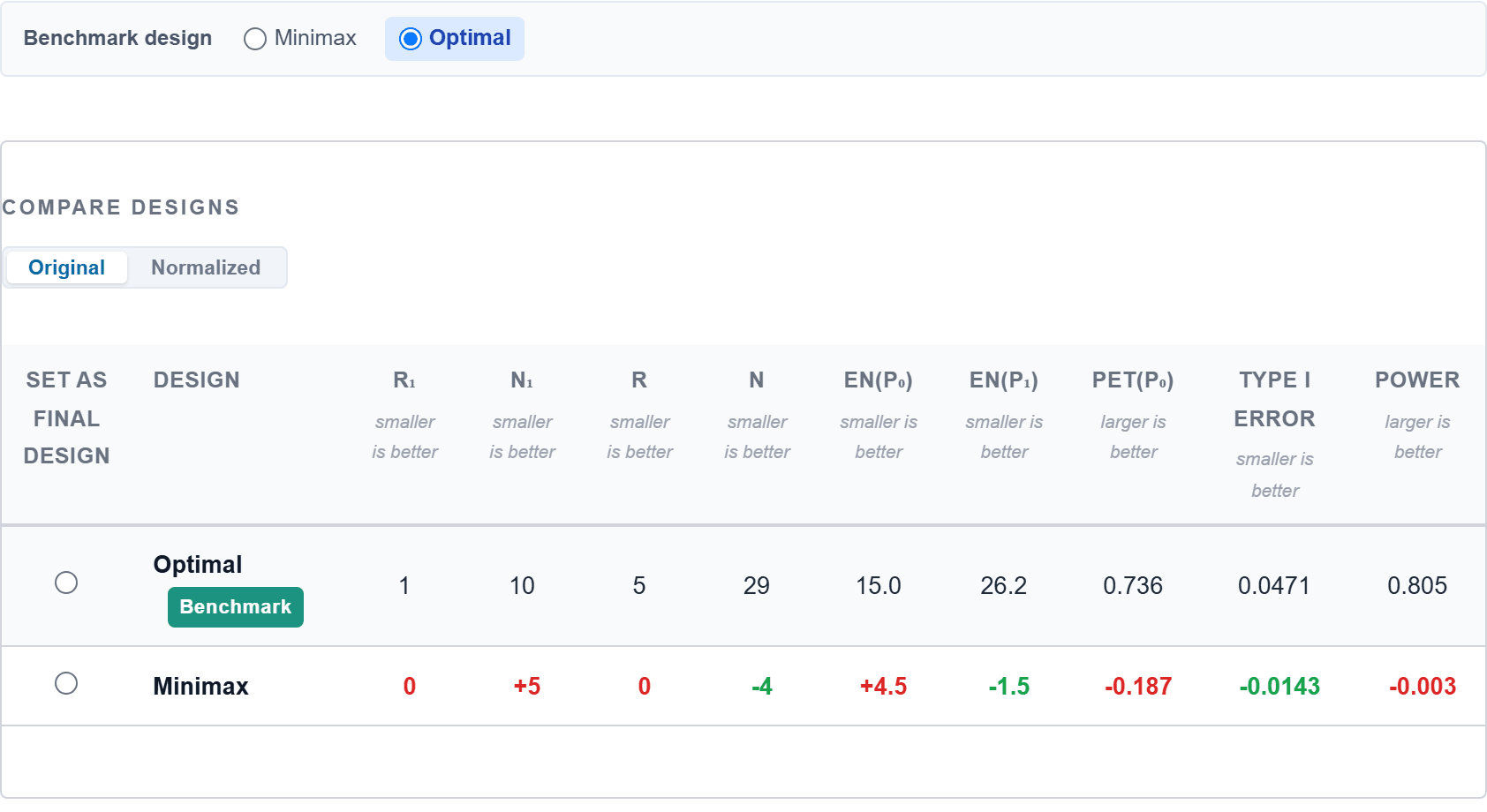
| Operating characteristic | Minimax | Optimal |
|---|---|---|
| Maximum sample size | 25 | 29 |
| PET under p₀ = 0.10 | 0.5490 | 0.7361 |
| Expected sample size under p₀ = 0.10 | 19.51 | 15.01 |
| Expected sample size under p₁ = 0.30 | 24.65 | 26.16 |
| Type I error | 0.0328 | 0.0471 |
| Power | 0.8017 | 0.8051 |
Why is EN(p₁) higher for the Optimal design?
The Optimal design has a higher expected sample size under the promising response rate. This is not a contradiction: the Optimal design minimizes expected sample size under the null hypothesis, not under every possible response rate. If minimizing expected enrollment when the treatment is promising matters to your trial, compare EN(p₁) explicitly.
Why are Type I error and power not exactly 0.05 and 0.80?
Simon designs use integer-valued sample sizes and response thresholds, so the attainable operating characteristics are discrete. A design is feasible when its actual Type I error is at most 0.05 and its actual power is at least 0.80. The search therefore identifies feasible designs rather than designs whose operating characteristics equal the requested values exactly.
The Optimal design has a Type I error of approximately 0.0471 and power of approximately 0.8051; both satisfy the requirements. The Minimax design has a lower Type I error of approximately 0.0328. This does not make it invalid: its defining objective is to minimize maximum sample size, not to use the entire Type I error allowance.
Why do all four designs have r₁ = 1?
All four designs use the same first-stage futility threshold: the trial stops if no more than one response is observed in Stage 1. The first-stage sample size and the number of additional Stage 2 patients differ, producing different probabilities of early termination and expected sample sizes.
The threshold is part of the complete decision rule and should not be interpreted independently of the other design parameters.
Understand PET and Expected Sample Size
Two operating characteristics are particularly useful when evaluating Simon designs: the probability of early termination (PET) and the expected sample size (EN). PET is the probability that the trial stops after Stage 1 because the observed number of responses is insufficient. Under a true response rate p:
For the Optimal design, n₁ = 10 and r₁ = 1. Under the unacceptable response rate, PET(0.10) = P(X₁ ≤ 1) ≈ 0.7361. When the true response rate is 10%, the trial has approximately a 73.6% probability of stopping after Stage 1.
PET should also be examined under p₁. A design should not be evaluated only by how frequently it stops when the treatment is ineffective; you also need to understand its behavior when the treatment is promising. For the Optimal design, PET(0.30) ≈ 0.1493, so about 14.9% of trials of a genuinely promising treatment would stop after Stage 1.
Expected sample size
The expected sample size under a true response rate p is EN(p) = n₁ + n₂ × [1 − PET(p)]. Every trial enrolls the first-stage patients; only trials that continue beyond Stage 1 enroll the additional Stage 2 patients.
For the Optimal design under p₀ = 0.10, EN(0.10) = 10 + 19 × (1 − 0.7361) ≈ 15.01. Although the maximum sample size is 29, the expected sample size under the null response rate is approximately 15 patients.
How are Type I error and power calculated?
The operating characteristics are calculated from the probabilities of the possible response counts in both stages. For the decision rule used here, the probability of declaring success at response rate p is the sum, over first-stage counts x₁ from r₁ + 1 to n₁, of P(X₁ = x₁ | p) × P(X₂ > r − x₁ | p), where X₁ ~ Binomial(n₁, p) and X₂ ~ Binomial(n₂, p).
When x₁ > r, the final success threshold has already been reached during Stage 1, so the second-stage probability factor is automatically equal to one.
The Type I error is this probability at p₀, and the power is this probability at p₁. This is why the complete decision rule must be evaluated: the first-stage stopping threshold, the second-stage sample size, and the final response threshold all contribute to the operating characteristics.
Choose the Appropriate Design
Which design should you select? The answer depends on your trial’s practical constraints.
| Your priority | Design to examine first | Reason |
|---|---|---|
| Minimize expected enrollment if the treatment is ineffective | Optimal | Minimizes EN(p₀) |
| Impose a strict maximum recruitment limit | Minimax | Minimizes maximum sample size |
| Find a compromise between maximum and expected sample size | Admissible | Balances N and EN(p₀) |
| Minimize expected enrollment when the treatment is promising | Compare EN(p₁) explicitly | This is not the Optimal design’s defining objective |
Applying the priorities to this example
Suppose recruitment is difficult and the clinical team wants to minimize unnecessary patient exposure when the treatment is ineffective. The Optimal design is attractive because it has a PET of approximately 73.6% under p₀ and an expected sample size of approximately 15.01.
Suppose instead that the trial has a strict enrollment ceiling of 25 patients. The Minimax design becomes more attractive because it guarantees that enrollment will not exceed 25 patients.
Neither choice is universally better. The right decision depends on the trial’s recruitment capacity, budget, patient population, and clinical priorities.
Document the Selected Design
Suppose the clinical team selects the Optimal design: n₁ = 10, r₁ = 1, n₂ = 19, N = 29, r = 5. The decision rule can be written as follows:
Enroll 10 patients in Stage 1. If one or fewer responses are observed, terminate the trial for futility. If two or more responses are observed, enroll an additional 19 patients. At the end of Stage 2, declare the treatment promising if at least 6 responses have been observed among all 29 patients.
Clicking the Optimal design in the candidate table opens its details; Set as Final Design records the selection. The corresponding operating characteristics are summarized below the figure.
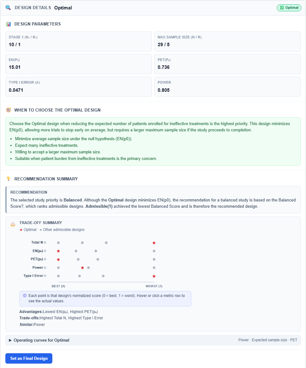
| Characteristic | Value |
|---|---|
| Type I error | 0.0471 |
| Power | 0.8051 |
| Maximum sample size | 29 |
| PET under p₀ | 0.7361 |
| Expected sample size under p₀ | 15.01 |
| Expected sample size under p₁ | 26.16 |
Practical Considerations and Limitations
Before implementing a Simon's two-stage design, consider several practical issues.
Account for dropout and unevaluable patients
The classical design is based on a specified number of patients with evaluable binary outcomes. If dropout or unevaluable outcomes are anticipated, the enrollment plan must account for them.
A common practical approximation is to inflate the planned stage sample sizes by a factor of 1 / (1 − d), where d is the anticipated dropout proportion, and to apply the original decision rule to the required number of evaluable patients.
This is an approximation, not a guarantee that the original operating characteristics are preserved. If dropout is substantial, potentially related to treatment response, or handled through a more complex replacement policy, assess the implications for Type I error and power, for example through simulation. The statistical analysis plan should explicitly define how missing and unevaluable outcomes are handled.
Plan the timing of the interim analysis
The first-stage decision should take place only when the required Stage 1 response data are sufficiently mature. In an oncology trial, response confirmation and assessment schedules can affect when the first-stage results become available. The operational plan should specify when Stage 1 is considered complete and when the futility decision can be made.
Classical Simon designs stop early for futility, not efficacy
A classical Simon's two-stage design allows the trial to stop after Stage 1 when the observed response count is insufficient. It does not include an early efficacy stopping rule. The treatment is declared promising only after completion of Stage 2 and evaluation of the final response threshold. If early efficacy stopping or additional interim analyses are required, a different design framework is needed.
Understand the scope of the design
The classical Simon design is a frequentist design intended primarily for single-arm Phase II trials with a binary endpoint. It assumes a prespecified response-rate model and a fixed two-stage decision rule.
It does not automatically accommodate multiple interim efficacy analyses, additional interim futility analyses at times other than the prespecified Stage 1 analysis, sample-size re-estimation, changes to the decision rule during the trial, or complex missing-data or competing-event mechanisms. Such features require additional statistical planning and potentially a different design methodology.
Explore Your Own Simon's Two-Stage Design
This example demonstrates how clinical assumptions translate into sample sizes and decision rules. Your own trial may have different response-rate assumptions, statistical requirements, and recruitment constraints, and changing p₀, p₁, Type I error, or power can lead to substantially different designs.
Generate and compare designs using your own trial assumptions rather than adopting the numerical example directly. Follow the BioStatHub step-by-step guide to generate and compare Simon designs, from entering the assumptions to exporting the design record.
Frequently Asked Questions
What parameters are needed to calculate a Simon's two-stage design?
The four principal inputs are the unacceptable response rate (p₀), the promising response rate (p₁), the Type I error (α), and the power (1 − β).
What is a Simon's two-stage design example with p₀ = 0.10 and p₁ = 0.30?
With Type I error 0.05 and power 0.80, the Optimal design is n₁ = 10, r₁ = 1, n₂ = 19, N = 29, r = 5. It has an expected sample size of approximately 15.01 under p₀ = 0.10 and a PET of approximately 0.7361. The corresponding final success threshold is at least 6 responses among 29 patients.
What is the difference between Optimal and Minimax Simon designs?
The Optimal design minimizes expected sample size under the null response rate, while the Minimax design minimizes the maximum total sample size. Both must satisfy the specified statistical constraints.
Can a Simon's two-stage design stop early for efficacy?
No. A classical Simon's two-stage design stops early for futility only. It declares the treatment promising after completion of Stage 2 if the final response threshold is met.
How do I account for dropout in a Simon's two-stage design?
The classical design is based on evaluable binary outcomes. A common approximation is to inflate the planned stage sample sizes by the anticipated dropout factor and apply the decision rule to evaluable patients. This should be assessed carefully because the original operating characteristics are not automatically preserved. The statistical analysis plan should specify how missing and unevaluable outcomes are handled.
Is the expected sample size the same as the maximum sample size?
No. Maximum sample size is the largest possible enrollment. Expected sample size accounts for the probability of stopping early and depends on the assumed true response rate.
Which Simon design should I choose?
There is no universally best design. The Optimal design emphasizes expected sample size under the null, the Minimax design emphasizes maximum enrollment, and Admissible designs offer compromises between the two. The final choice should reflect the trial’s clinical and operational priorities.